Probit - Theory

Last week, we encountered linear regression analysis which allowed us to quantify the amount and direction of one or more independent variables on a continuous dependent variable. I already mentioned there, that there is also a type of a regression which can deal with a binary dependent variable. This is usually a yes/no scenario, such as democracy / autocracy, war / peace, trade agreement / no trade agreement, … You get the picture. Many problems or questions in political science have binary outcomes, and so you are about to learn a very important and useful method to answer research questions. As in the previous Chapter, I will take you some through some theory first, and then we are applying the theory to an empirical example. This time concerning the survival of passengers on the Titanic.

Probit - What is it?

A question we can all relate to is whether to go out tonight, or not. The “propensity to go out” is not directly observable, and so we call this a latent variable. You can imagine this running from minus infinity to plus infinity, and at some point on this continuum you are making the decision to go out. Let’s call this point tau (\(\tau\)). Graphically, this would look like this:

Figure 8: Latent Variable

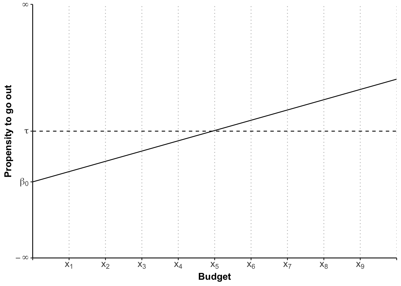
Your inclination to go out, is likely to be influenced by the amount of money you have in your wallet / bank. If you are broke, you will be less inclined (if you are sensible), and if you are swimming in it, you will be more inclined. So, if the “propensity to go out” (which remember is running from minus to plus infinity) is influenced by your budget, then let’s construct a graph, in which we pop the propensity to go out on the y-axis, and the budget on the x-axis. If we assume that this relationship is linear, we can fit a regression line into this coordinate system, just as we have in the previous week:

Figure 9: Effect of Budget on Propensity to Go Out

Whilst this visualises the influence of the budget on the latent variable, what we are aiming for is to make a prediction about the probability of you going out, or not.

Now imagine, your budget is \(x_{1}\). The regression line depicts the propensity that we would expect to see, on average, for somebody with a budget of \(x_{1}\). But the crucial point is that not everybody is average. Some might have an essay deadline approaching which makes them even less likely to go out. Others might just have recieved their essay mark, and want to celebrate that they scored a first. In other words, there is variability around the regression line. And we assume that whilst this variability is random, it still follows a particular distribution. In the case of a probit, this is the normal distribution⁴. I have added these distributions to Figure 10. As you can see, even at budget \(x_{1}\), some area of the distribution has slipped over the cut-off point, \(\tau\).

Figure 10: Towards the Cumulative Density Function, adapted from J. S. Long (1997, p. 46)

The probability of going out is coloured in in grey. You can see that even at \(x_{1}\) there is a teeny bit of probability that you will go out. As the budget increases, more and more probability slides over the threshold \(\tau\), until we reach the magical point of \(x_{5}\) where the probability is 50%. From there on, the amount of probability sliding over \(\tau\) is steadily decreasing, because of the shape of the normal distribution.

We can depict the amount of probability (or the size of the grey area) for each \(x_{i}\) in a separate graph which is called the Cumulative Probability Density Function, or short CDF:

Figure 11: The Cumulative Distribution Function, adapted from J. S. Long (1997, p. 46)

This s-shaped curve now gives us the probability (of going out) for each \(x_{i}\) (budget). It is important to note that the relationship is not linear, as in linear regression. Because we have an s-shaped curve the increase in probability when going from \(x_{2}\) to \(x_{3}\) is not the same as going from \(x_{3}\) to \(x_{4}\). You can see that visualised here:

Figure 12: Marginal Effect under the Cumulative Density Function

We will therefore not be able to interpret the coefficients in the same way as for OLS. We will be using predicted probabilities instead. But one step at a time. Let’s first get our hands dirty with some data.

---

4. For logit, the logistic distribution is used. This would lead to very similar results.↩︎