Linear Regression - Theory
Introduction
Regression is the power house of the social sciences. It is widely applied and takes many different forms. In this Chapter we are going to explore the linear variant, also called Ordinary Least Squares (OLS). This type of regression is used if our dependent variable is continuous. In the following Chapter we will have a look at regression with a binary dependent variable and the calculation of the probability to fall into either of those two categories. But let’s first turn to linear regression.
What is it?
Regression is not only able to identify the direction of a relationship between an independent and a dependent variable, it is also able to quantify the effect. Let us choose Y as our dependent variable, and X as our independent variable. We have some data which we are displaying in a scatter plot:

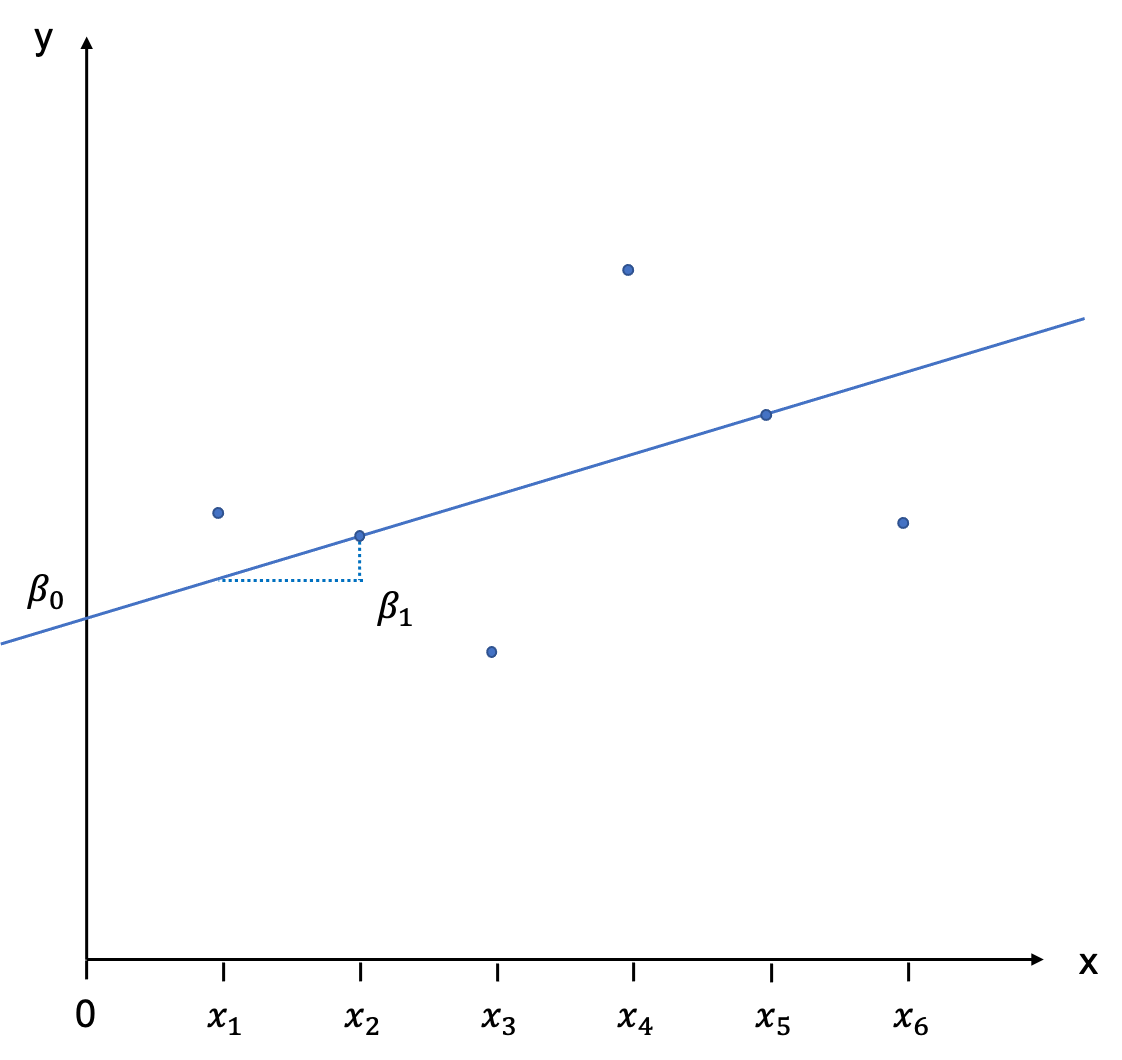
With a little goodwill we can already see that there is a positive relationship: as X increases, Y increases, as well. Now, imagine taking a ruler and trying to fit in a line that best describes the relationship depicted by these points. This will be our regression line.
The position of a line in a coordinate system is usually described by two items: the intercept with the Y-axis, and the slope of the line. The slope is defined as rise over run, and indicates by how much Y increases (or decreases is the slope is negative) if we add an additional unit of X. In the notation which follows we will call the intercept \(\beta_{0}\), and the slope \(\beta_{1}\). It will be our task to estimate these values, also called coefficients. You can see this depicted graphically here:
In the context of the module, we would for example have per capita GDP on the x-axis (independent variable), and Polity V measuring the level of democracy on the y-axis (dependent variable). This would look like this in the year 2015:
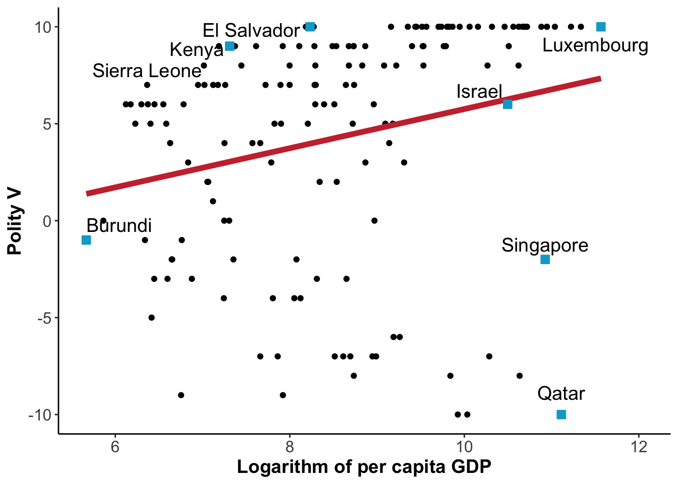
Figure 7: Democracy and Development in 2015
Population
We will first assume here that we are dealing with the population and not a sample. The regression line we have just drawn would then be called the Population Regression Function (PRF) and is written as follows:
\[\begin{equation} E(Y|X_{i}) = \beta_{0} + \beta_{1} X_{i} \end{equation}\]
Because wer are dealing with the population, the line is the geometric locus of all the expected values of the dependent variable Y, given the values of the independent variables X. This has to do with the approach to statistics that underpins this module: frequentist statsctics (as opposed to Bayesian statistics). We are understanding all values to be “in the long run”, and if we sampled repeatedly from a population, then the expected value is the value we would, well, expect to see most often in the long run.
The regression line is not intercepting with all observations. Only two are located on the line, and all others have a little distance between them and the PRF. These distances between \(E(Y|X_{i})\) and \(Y_{i}\) are called error terms and are denoted as \(\epsilon_{i}\).
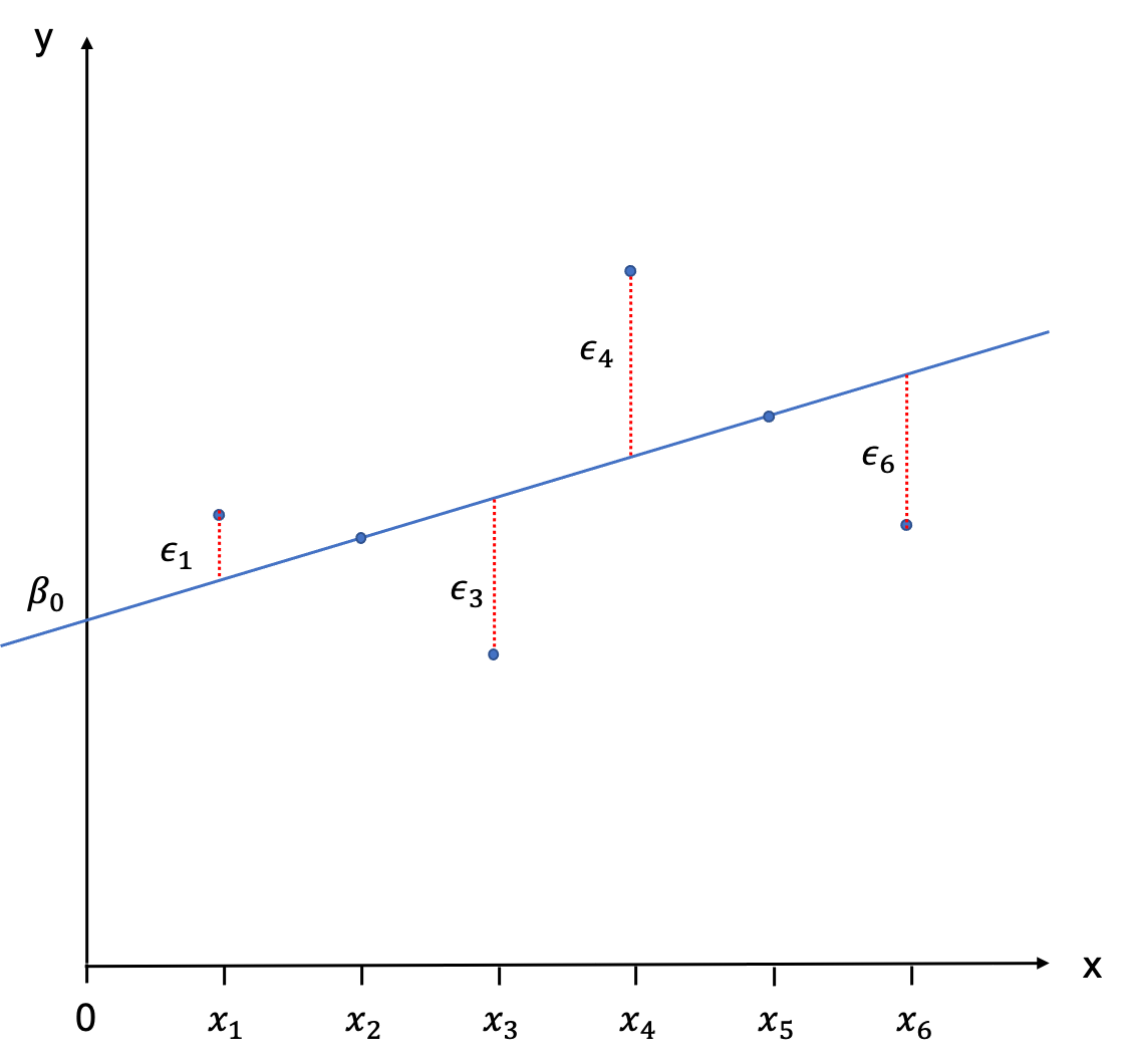
To describe the observations \(Y_{i}\) we therefore need to add the error terms to the PRF:
\[\begin{equation} Y_{i} = \beta_{0} + \beta_{1} X_{i} + \epsilon_{i} \end{equation}\]
Sample
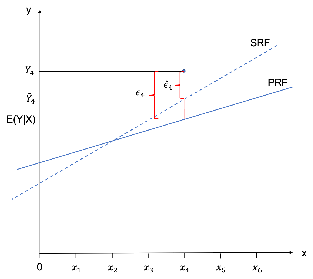
In reality we hardly ever have the population in the social sciences, and we generally have to contend with a sample. Nonetheless, we can construct a regression line on the basis of the sample, the Sample Regression Function (SRF). It is important to note that the nature of the regression line we derive fromt he sample will be different for every sample, as each sample will have other values in it. Rarely, the PRF is the same as the SRF - but we are always using the SRF to estimate the PRF.
In order to flag this up in the notation we use to specify the SRF, we are using little hats over everything we estimate, like this:
\[\begin{equation} \hat{Y}_{i} = \hat{\beta}_{0} + \hat{\beta}_{1} X_{i} \end{equation}\]
Analogously, we would would describe the observations \(Y_{i}\) by adding the estimated error terms \(\hat{\epsilon}_{i}\) to the equation.
\[\begin{equation} Y_{i} = \hat{\beta}_{0} + \hat{\beta}_{1} X_{i} + \hat{\epsilon}_{i} \end{equation}\]
The following graph visdualised the relationship between an observation, the PRF, the SRF and the respective error terms.
Ordinary Least Squares (OLS)
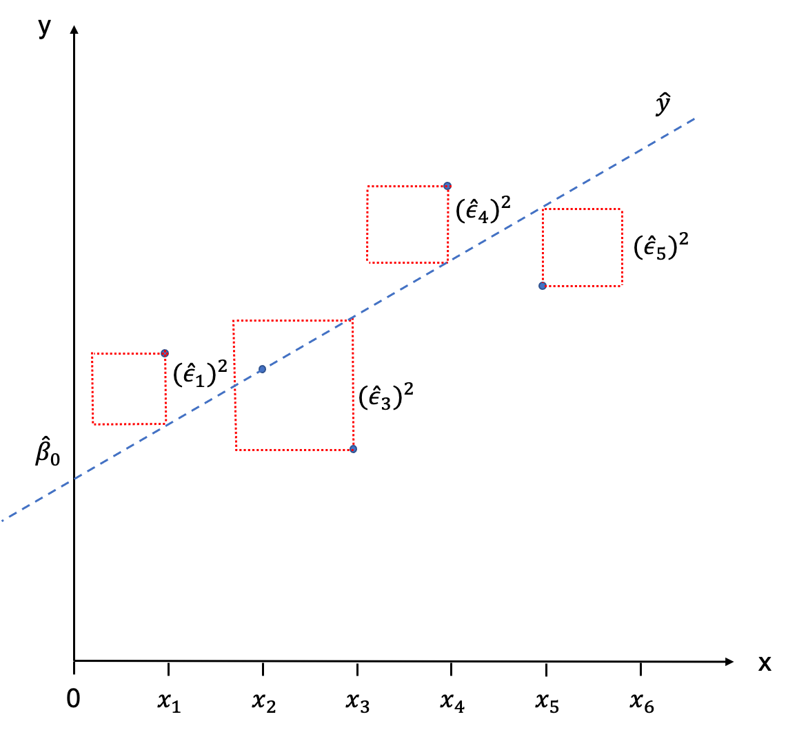
When you eye-balled the scatter plot at the start of this Chapter in order to fit a line through it, you have sub-consciously done so by minimising the distance between each of the observations and the line. Or put differently, you have tried to minimise the error term \(\hat{\epsilon}_{i}\). This is basically the intuition behind fitting the SRF mathematically, too. We try to minimise the sum of all error terms, so that all observations are as close to the regression line as possible. The only problem that we encounter when doing this is that these distances will always sum up to zero.
But similar to calculating the standard deviation where the differences between the observations and the mean would sum up to zero (essentially we are doing the same thing here), we simply square those distances. So we are not minimising the sum of distances between observations and the regression line, but the sum of the squared distances between the observations and the regression line. Graphically, we would end up with little squares made out of each \(\hat{\epsilon}_{i}\) which gives the the method its name: Ordinary Least Squares (OLS).
We are now ready to apply this stuff to a PO3B3-related example!