Introduction to R
How Data are organised
I have put a little sample data set together for you which you can see here:
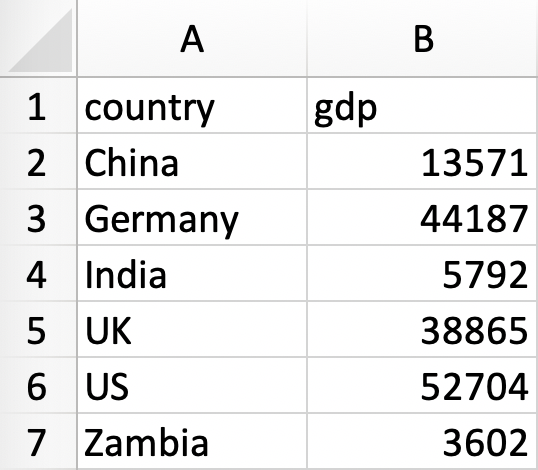
Figure 1: Sample Data Set
Each column represents a variable, the first one country names, and the second per capita GDP in 2015. Each row represents an observation, in our case an individual country. The meeting point between the the variable and the observation is a particular value. So for example, in Figure 1 the GDP (second column) of the third country (row) is $ 5792 (cell). You see in the first row the names of the variables. Always make these short and sweet, but especially telling. Don’t go for something like “x4_st”, or “fubar”, as nobody (including yourself after a little while) will have any clue what this is.
R & RStudio – Installation
Now we are ready to start working with R. The first step is to install the program. Please follow these instructions:
- Go to https://cran.r-project.org/mirrors.html and select a server from which you want to download R. It is convention to do this from the server which is nearest to you. Follow on-screen instructions and install the program.
- Go to https://rstudio.com/products/rstudio/download/ and download RStudio Desktop which is free. Install the program.
- Now open RStudio.
Whilst you need to install both R and RStudio, we will never be working with R directly. Instead, we will be operating it through RStudio.
R - Getting Started
In this companion I am using two different fonts:
- Font for plain text
A typewriter font for R functions, values, etc.
Let’s have a look at RStudio itself. When you open the programme, you are presented with the following screen:
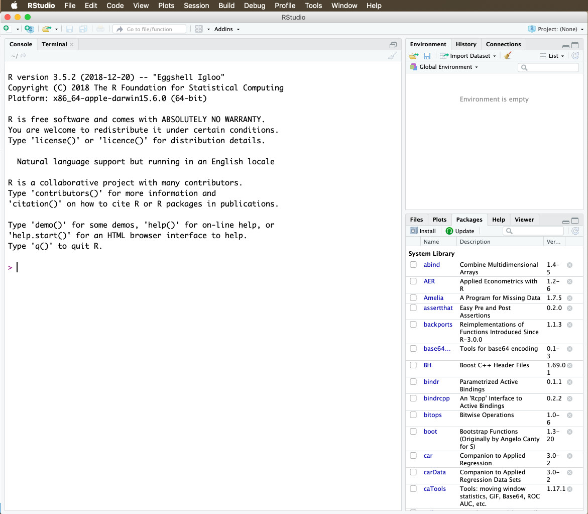
Figure 2: RStudio
It has – for now – three components to it. On the left hand-side you see the so-called “Console” into which you can enter the commands, and in which also most of the results will be displayed. On the right hands side, you see the “Workspace” which consists of an upper and a lower window. The upper window has three tabs in it. The tab “Environment” will provide you with a list of all the data sets you have loaded into R, and also of the objects and values you create (more on that later). Under the “History” tab, you find a history (I know, who would have thought it) of all the commands you have used. This can be very useful to retrace your steps. In the “Connections” tab you can connect to online sources. We will not use this tab.
In the lower window, you have five tabs. Under “Files” you find the file structure of your computer. Once you have set a working directory (more on that in a moment), you can also view the files in your working dorectory here which gives you a good overview of the files you need to refer to for a particular project. The “Plots” tab will display the graphs we will be producing. “Packages” form the heart and soul of R and they make the program as powerful as it is (again, more on that later). RStudio also has a “Help” function, which is rarely very illuminating. I usually search for stuff online on “stackexchange”, as there is a large community of R users out there who share their knowledge and solutions to problems. We won’t use the last tab “Viewer”.
RScript
If you read the previous section carefully, you will have noticed that I wrote that you can enter the commands” in the Console. You can, but you shouldn’t. What you should be using instead is an RScript. An RScript is a list of commands you use for a project (an essay, your dissertation, an article) to calculate quantities of interest, such as descriptive statistics in the form of mean, median and mode, and produce graphs.
One of the foundations of scientific research is “reproducibility”“, or”replicability”. This means that “sufficient information exists with which to understand, evaluate, and build upon a prior work if a third party could replicate the results without any additional information from the author.” (King, 1995, p. 444, emphasis removed) This principle applies in academia more generally, because only if you understand what a person has done before you, you can pick their work up whether they left it, and push the boundaries of knowledge further. But a bit closer to home, it is also relevant for conducting quantitative research in assessments. We require you to submit an RScript (or a “do file” if you use Stata) now together with your actual essay. This is not only to check what you have done; data preparation is often the most time-consuming part (as you will soon discover), and this is a way to gain recognition for this work. So it is actually to your advantage, and not a mere plagiarism check.
The creation of an RScript will allow you to open the raw data, and by running the script, to bring it to exactly where you left off. This saves you saving data sets which can take up a lot of work. If you back the script up properly, you also have an insurance against losing all your work a day before the assessment is due.
To create an RScript, click File → New File → RScript. A fourth window opens, and your screen will now look something like this:
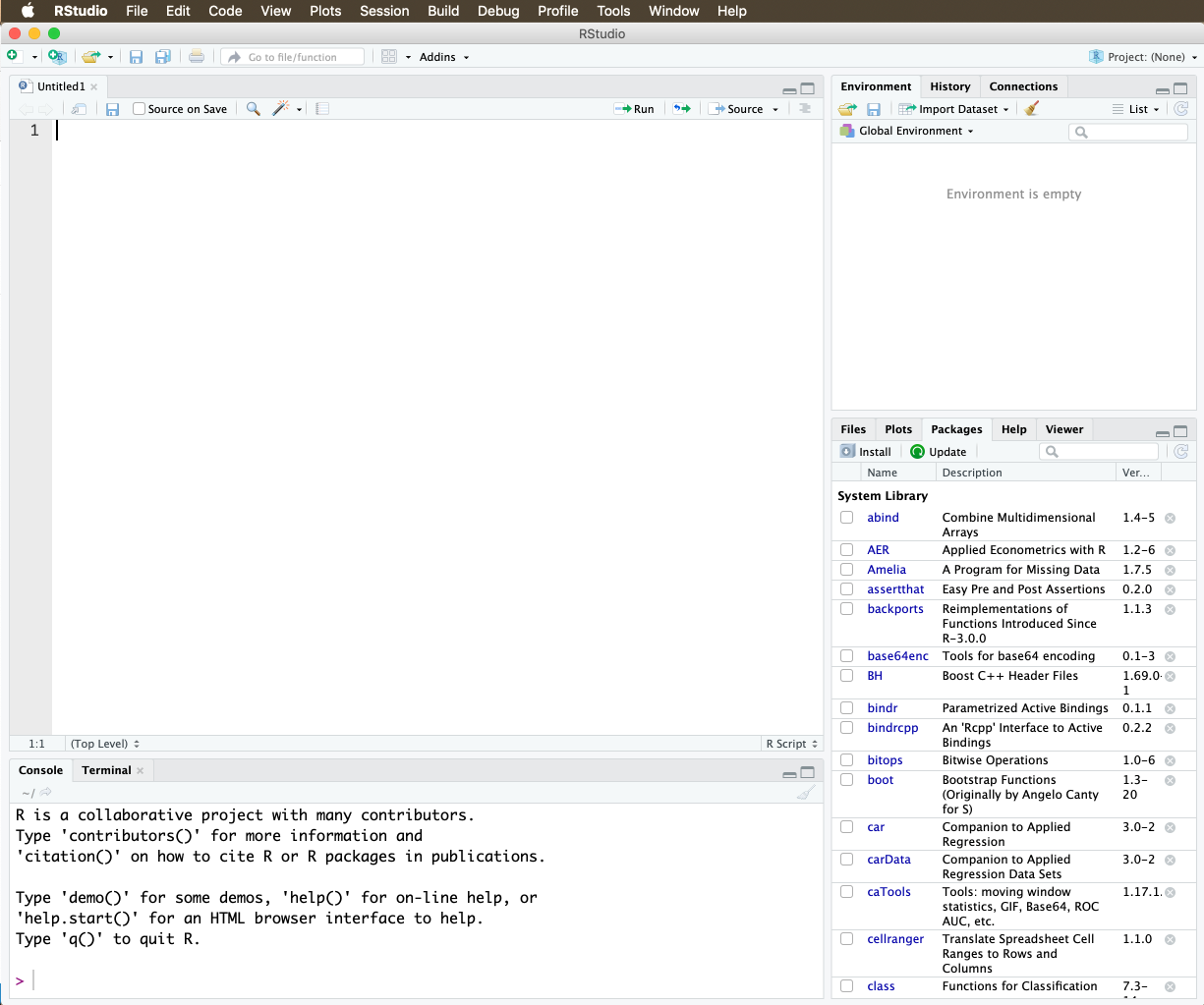
Figure 3: The RScript Window
You can now write your commands in the RScript, where a new line (for now) means a new command. If you want to execute a command, put the cursor on the line the command is on and press “command” / “enter” simultaneoulsy on a Mac and “Ctrl” / “Enter” on Windows.
If you precede a line with #, you can write annotations to yourself, for example explaining what you do with a particular command. More on this in the next sub-section.
Figure 4 shows the start of the RScript for this worksheet. I prefer a dark background, it’s easier on the eyes, especially when you work with R for long periods. You can change the settings in: Tools → Global Options → Appearance → Twilight.
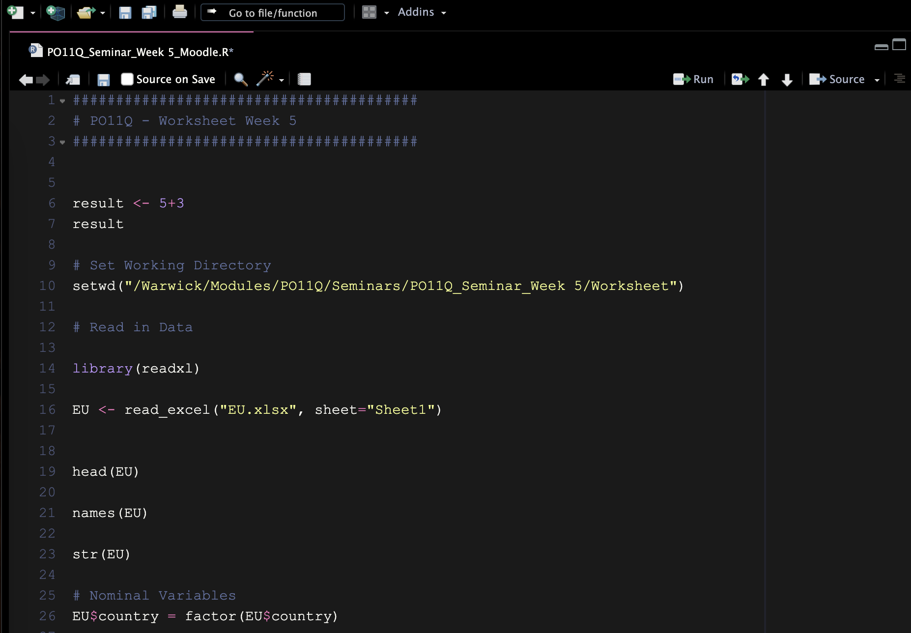
Figure 4: Example of an RScript
More Themes
If you copy and paste the following code chunks into your “Console” and run one at a time, you will have even more themes1 to choose from:
install.packages(
  "rsthemes",
  repos = c(gadenbuie = 'https://gadenbuie.r-universe.dev', getOption("repos"))
)You can also download Flo’s Dark Theme2 and then “add” it at the bottom of the “Appearance” menu.
RScript Structure
Well, I am German, and I like things neat and tidy, so I feel almost compelled to discuss how to properly organise an RScript. But apart from genetical dispositions, a well-organised RScript is also very much in the spirit of reproducibility. It simply makes sense to structure an RScript in such a way that another researcher is able to easily read and understand it.
First of all, which commands to include? If you introduce me to your current girlfriend or boyfriend, I have no interest in learning about all your past relationships; they have not worked out. In a similar fashion, nobody wants to read through lines of code that are irrelvant. So you will only include in the RScript those commands which produce the output you actually include in the essay or article.
I stated above that if you precede a line with #, you can write annotations to yourself. This is also a useful way to structure an RScript, for example into exercise numbers, sections of an essay /article, or different stages of data preparation (which we will be doing in due course).
Now you know how to write in an RScript, avoid using the “Console” to write your code, and only write in the RScript.
First Steps in R
But enough of the preliminary talk, let’s get started in R. In principle, you can think of R as a massive and powerful calculator. So I will use it as such to start of with. If you want to know what the sum of 5 and 3 is, you type
and press “command” / “enter” (or “Ctrl” / “enter” if you are on Windows). In everything that is to follow, commands will be shown in boxes with the output underneath preceded by a hash tag. So, including result, the calculation would look like this:
where the [1] indicates that the 8 is the first component of the result. In this case, we only have one component, so it’s superfluous really, but we will soon encounter situations in which results can have a number of different items. Note that the result of this operation is displayed in the “Console”, even if you write this in the RScript above.
You can copy the code from this page by hovering over the code chunk and clicking the icon in the top-right hand corner. You can then paste it into your RScript.
A fundamental component of R is objects. You can define an object by way of a reversed arrow, and you can assign values, characters, or functions to them. If we want to assign the sum of 5 and 3 to an object called result, for example, we call3
If we now call the object, R will return its value, 8.
The Working Directory
It is imperative that you create a suitable filing system to organise the materials for all of your modules. At the very least you should have a folder called “University” or similar, in which you have a sub-folder for each module you take.
In those modules in which you are working with R, you need to extend this system a little. I have created a schematic of what I have in mind in Figure 5.
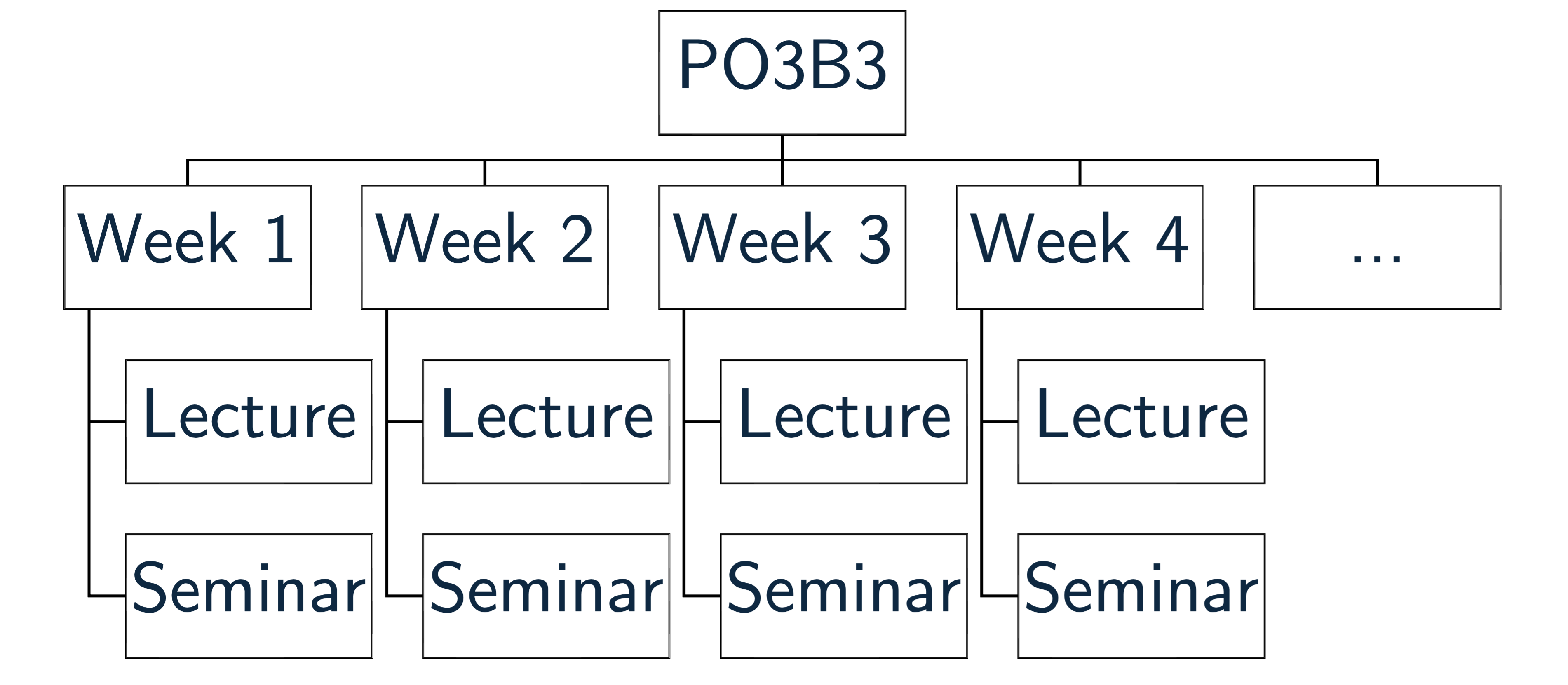
Figure 5: Folder Structure
You see that there is a sub-folder for each week of the module (I have only done a few for illustrative purposes), and that each of these folders is divided into lecture and seminar in turn. Into these you can place the lecture and seminar materials, respectively. Create this system now for PO3B3.
R works with so-called “Working Directories”. You can think of these as drawers from which R takes everything it needs to conduct the analysis (such as the data set), and into which it puts everything it produces (such as graph plots). As this will be an R-specific drawer within the seminar, create yet another sub-folder in your seminar folder, and call it something suitable, such as “PO3B3Q_Seminar_Week 1”. Do NOT call this “Working Directory”, as you will have many of those, rendering this name completely meaningless.
Please set up this structure now. If I find you using a random folder on your desktop named “working directory” in the coming weeks, I am going to implode! I mean it.
Now we need to tell R to use this folder. If you know the file structure of your computer you can simply use the command, and enter the path. Here is an example from my computer:
If you don’t know the file structure of your computer, then you can click Session → Set Working Directory → Choose Directory.
R Packages
It would be difficult to overstate the importance of packages in R. The program has a number of “base” functions which enable the user to do many different basic things, but packages are extensions that allow you to do pretty much anything and everything with this software - this is one of the reasons why I love it so much. The first package we need to use will enable us to load an Excel sheet into R. It is called readxl. You can install any package with the command install.packages() where the package name goes, wrapped in quotation marks, into the brackets:
We can then load this package into our library with the library() command.
Once you close R at the end of a session, the library will be reset. When you reopen R, you have to load the packages you require again. But you do not have to install them again.
Working with Your Data Set
Opening
We are now ready to open the data set in R - where it is called a “data frame”. First, download the Example data set (also available in the Downloads Section) and place it into the current working directory. To load it into R, we create a new object example, and ask R to read “Sheet 1 of the Excel file”example.xlsx”.
Please do not use the “Import Dataset” button in the Environment, but do this properly, manually. We sometimes need to set options for importing data sets, and the “pointy, clicky” approach won’t be able to offer you what you need.
We can now use our data in R!
Viewing the Data
In the present case, you know what the data look like, but very often when you use secondary data sets, you don’t. So it’s a good idea to view the data frame before doing anything with it. To view the data frame in a way you might be familiar with from Excel (even though you cannot edit this in the same way). apply the View() command.
If you only want to see the first 6 observations of each variable, use the head() command:
head(example)
# A tibble: 6 × 2
  country   gdp
  <chr>   <dbl>
1 China   13571
2 Germany 44187
3 India    5792
4 UK      38865
5 US      52704
6 Zambia   3602
If you simply want to know the variable names in the data frame, type:
The next one is a very important command, because it reveals not only the variable names and their first few observations, but also the nature of each variable (numerical, character, etc.). It is the str() command, where “str” stands for structure:
Variable Types in R
You have seen in the output of the str() command that R distinguishes between a number of different variable types. Here is a broad overview of the variable types, so that you know which descriptive statistics you can calculate, or into which variable type you need to recode (next step) to achieve what you want. There are two general types:
numeric– numberscharacter(also called string) – letters
Within numeric we can distinguish between the following:
factor- nominal variableordered factor- ordinal variableinteger- numeric, but only “whole” numbers (discrete)numeric- any number (interval or ratio scales)
If you are unfamiliar with measurement scales, then please look these up before proceding.
Descriptive Statistics
Quite a large number of descriptive statistics can be calculated. For example:
- Mean
- Median
- Mode
- Range
- Standard Deviation
- Variance
Again, if these don’t mean anything to you beyond having heard the term before, please look these up.
They are a lot of effort to calculate by hand, especially for larger data sets, but R can do these with a few intuitive commands. If we want to refer to a particular column in R (which is equivalent to a variable), then we need to specify the data frame within which the variable is located, followed by a $ sign and then the variable name. Schematically, this would look be written as dataframe$variable.
With this information to hand, we can calculate the mean of the variable gdp:
Then the median:
Mean, median, and also mode (the most frequently occurring value) are all measures of centrality, but centrality alone does not adequately describe a distribution. You can think of two scenarios, in both we have two people in a group and we are trying to describe their age. In group one we have one person who is 50 years old, and one who is 52 years old. Average age = 51. In the second group we have a toddler aged 2, and a very old person aged 100. Same average, but a very different distribution of age. Schematically you can see this in Figure 6 where two distributions have the same mean, median and mode, but their spread is quite different.
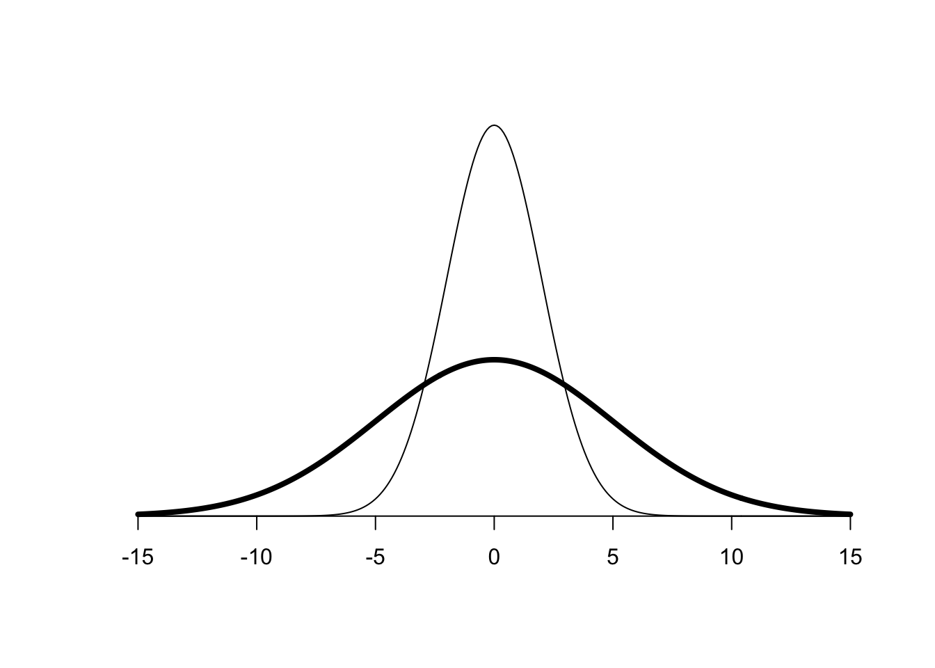
Figure 6: Distributions with different Standard Deviations
Therefore, we also need to look at the variability of a variable to adequately describe it. Again, there are quite a few measures available. First up is the range; you can either calculate this with two commands by finding out the minimum and maximum separately, or just ask R to give you the range straight away:
The standard deviation is rather long-winded to calculate by hand, but the R command is short and sweet:
The variance is the squared standard deviation, but you can calculate it with its own command in R, too:
You can get information on the quartiles (these are also measures of spread), the mean, as well as the minimum and maximum of a variable through one, simple command:
Data Manipulation
Recoding
When conducting quantitative research, variables will rarely come in the format in which you require them to be. I have been kind and reshaped all data you will be using for this module already. Nonetheless, you might come into a position in which you need to recode a variable, and here is how to do it.
The process is a little more involved, and requires a new package to be installed and loaded: dplyr. This package is part of the so-called tidyverse which is a suite of packages designed to make working with R simpler and commands shorter. You can install all of them by calling install.packages("tidyverse"). Let’s go all out with the tidyverse:
Now we can recode. Let’s say we want to create a new variable with two categories: low income and high income, where the cut-off sits at $ 20,000. The comnand to do this takes a little explaining. We start by stating the dataframe we wish to work with, example. The symbol which follows, %>%, reads as “and then”, and is called (yes seriously) a pipe. So we take the data frame example “and then” carry out a function called mutate. This function in turn defines the new variable gdpcat by recoding the variable gdp. The command then specifies all categories of the “old” variable gdp and what their respective values in the “new” variable gdpcat are going to be. The categories in each are set in quotation marks, as they are factor / character categories. The last step is then to assign this newly created variable gdpcat to our data frame example.
example %>%
  mutate(gdpcat=
           ordered(
             cut(gdp, breaks=c(0, 20000, Inf),
                 labels=c("low","high")))) -> example
Make a habit of adding a note underneath each of the more complex code chunks in your RScript (preceded with a #) in which you translate the code into plain English.
Let us now check the structure of the new variable to make sure that we have done everything correctly.
In my case all looks fine - make sure yours looks the same.
The Real Data Set
Download the world.csv data set from the Downloads Section and place it into the current working directory.
The data are taken from World Bank (2024), Boix et al. (2018), and Marshall & Gurr (2020). Table 1 provides a full code book, but you can also download it in pdf format here.
| variable | label |
|---|---|
| countrycode | Country Code |
| country | Country Name |
| year | Year |
| polity5 | Combined Polity V Score |
| democracy | 0 = Autocracy, 1 = Democracy (Boix et al., 2018) |
| gdppc | GDP per capita (current US Dollars) |
| enrol_gross | School enrollment, primary (% gross) |
| primcomp | Primary completion rate (% of relevant age group) |
| primcom_male | Primary completion rate, male (% of relevant age group) |
| primcom_fem | Primary completion rate, female (% of relevant age group) |
| enrol_net | School enrollment, primary (% net) |
| agri | Agriculture, forestry, and fishing, value added (% of GDP) |
| slums | Population living in slums (% of urban population) |
| telephone | Households with telephones (Landline & Mobile, %) |
| internet | Individuals using the Internet (% of population) |
| tax | Tax revenue (% of GDP) |
| pop | Population, total |
| pop_fem | Population, female (% of total population) |
| electricity | Access to electricity (% of total population) |
| service | Services, value added (% of GDP) |
| oil | Oil rents (% of GDP) |
| natural | Total natural resources rents (% of GDP) |
| literacy | Literacy rate, adult total (% of people ages 15 and above) |
| lit_male | Literacy rate, adult male (% of males ages 15 and above) |
| lit_fem | Literacy rate, adult female (% of males ages 15 and above) |
| infant | Mortality rate, infant (per 1,000 live births) |
| health_ex | Current health expenditure (% of GDP) |
| hospital | Hospital beds (per 1,000 people) |
| tuberculosis | Incidence of tuberculosis (per 100,000 people) |
| life | Life expectancy at birth, total (years) |
| life_male | Life expectancy at birth, male (years) |
| life_female | Life expectancy at birth, female (years) |
| unemploy | Unemployed (%) |
| urban | Urban population, total (% of total population) |
| attend | Births attended by skilled health staff (% of total) |
| prenatal | Pregnant women receiving prenatal care of at least four visits |
| military | Military Expenditure (% of GDP) |
| un_continent_name | Continent |
| un_region_name | Region on continent |
Again, let’s explore the data set through the view() function:
Now, don’t panic. This data set is big, but you know the basic structure: country by year in rows, and the variables in the column. The value for the variable in a given country in a given year is in the meeting point between row and column.
The data are (yes, the word “data” is plural) organised by country name in the first instance. So the first country you see is Afghanistan. There are multiple rows for Afghanistan, because each row gives you information about the value in a particular year (second column). This is repeated for every country in the world, leading to a total of 9.456 observations, to save you scrolling all the way down. Schematically, the structure of this data set looks as follows:
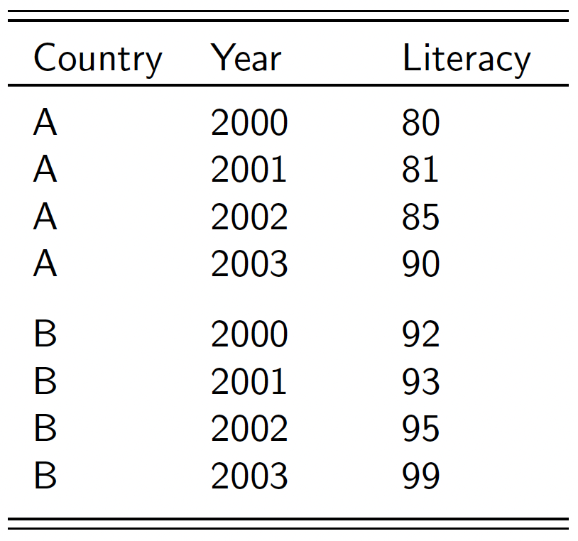
When you look at the data set in R, you will see that not every box contains a value - this means that the data are missing for this particular country-year for that particular variable. This is an issue we will be discussing a later stage in more detail, but I can already say now, that this issue is more pronounced in developing countries than in developed ones, and that it often severely limits the variables you can include in the analysis.
Let us conclude today with some more descriptive statistics to get used to entering and executing commands. Say, we want to find out the average GDP per capita of the UK since 1960 (which is when this data set begins, it ends in 2015). To do this, we first need to create a data frame which only contains data for GB. We call this process “subsetting”. The filter function comes out the dplyr package, and takes a particular data frame and filters all those observations which meet the condition specified. We will use this a lot on this module, and so it makes sense to remember this one well:
We can now produce
and all other descriptive statistics outlined before for “Great Britain”. If you want the number of observations, then you can display them by calling:
In this particular case, it would tell us that we have data for 56 years.
If this all seems a little much at the moment, don’t worry. As we go through the module, R will become much, much easier to handle!
Book Recommendations
If you want some more material to read up on R, then these are my recommendations:
- Fogarty (2023): The best applied R book on the market until my own book comes out.
- Stinerock (2022): Popular with students for good reasons!
- J. D. Long & Teetor (2019): Some recipes to cook with R
Please consult the List of References for full details.
This is a variation of the Dracula Theme.↩︎
To “call” means to execute a command.↩︎