Introduction to Matrices
What is a Matrix?4
The word “matrix” generally conjures up levels of horror in students which even Stephen King would be struggling to match5. And I have to admit that I have not always been best friends with them myself, either. But they are useful, and in their ability to convey a large amount of information in a structured and logical way, they are even beautiful. Because at the end of the day, a matrix is nothing more than a list.
In the lecture I introduced you to the concept of the Population Regression Function (PRF) which can be written as:
yi=β0+β1xi+ϵi
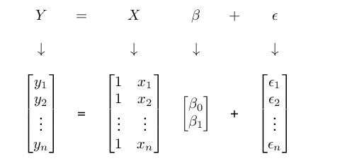
If we wanted to write out this equation for every observation in our data set, it would look something like this:
y1=β0+β1x1+ϵ1y2=β0+β1x2+ϵ2⋮yn=β0+β1xn+ϵn
This is incredibly wasteful, as it unnecessarily repeats notation. What we could do instead is to create a list which has as many columns as there are unique elements in these equations (since they all have the same structure), and only note the numeric values which actually change. And there you have a matrix:

Whilst this is what we will be using matrices for next week, let us leave regression aside for now, and focus on working with matrices more generally. We will now be using these two sample matrices:
A=[173954]B=[638232141539]
Matrix Notation
We can refer to individual elements of a matrix by stating the name of the matrix, and then in the index first the row, followed by the column (you might recognise this logic from R – this is because it is the same). With respect to matrix A, for example, the value in the first row and first column (1) would be referred to as
A11=1
The number in the first row, but second column would be referred to as
A12=7
What is the value of B23?
Calculating with Matrices
We will only need to multiply and divide matrices on this module, so let’s cover these operations now.
Multiplying Matrices
To show you how this is done, I will multiply matrix A with matrix B and record the results in a new matrix called C.
A×B=C=[173954]×[638232141539]=[3032245173578974]
In order to calculate a new element Ci,j, we multiply the elements of the ith row of A with the elements of the jth column of B. We then add together these so-called inner products in order to arrive at Ci,j. Let me give you some examples in which I have set the values from matrix A in bold to make the process more transparent.
C11=1×6+7×3+3×1=30
C12=1×3+7×2+3×5=32
C21=9×6+5×3+4×1=73
I have prepared a short video taking you through this process step by step. I would encourage you to watch it now.
If you can’t get enough of my delightful German accent, then I have some videos for you in which I go through the respective operation with matrices on screen. Here is the first:
Multiplying Matrices
Assume we are multiplying a 4x3 matrix with a 3x4 matrix with one another. How many rows and columns does the resulting matrix have?
Dividing Matrices
In order to be able to divide by an entire matrix, we take its inverse, and then multiply with the inverse6. We do the same in the non-matrix world. For example, if we wanted to divide 6 by 3, this is the same as multiplying 6 with 13, the inverse of 3. Sadly, inverting a matrix is not quite as straightforward as this. In fact, it is one of the most challenging operations you can do with a matrix. Luckily, the inversion of a 2 by 2 matrix (which is what we will be using) is still possible without a degree in algebra. The inverse D−1 of a 2 by 2 matrix D is defined as
D−1=[abcd]−1=1ad−bc[d−b−ca]−1
Thus, to arrive at the inverse of a 2 by 2 matrix, we first have to form the fraction in front of it. This takes as its denominator the difference between the products of the diagonal elements. We also refer to the denominator as the determinant of the matrix. In a second step – now in the matrix itself – we swap a and d, and set a minus sign in front of b and c.
Dividing Matrices
Special Matrices
There are two types of matrices we will be using which hold special, useful properties. This is the transpose of a matrix, and the so-called identity matrix.
Transposing Matrices
Another important operation is transposing a matrix, which turns rows into columns and columns into rows. We denote a transposed matrix with an apostrophe. Transposing matrix A into matrix A′ gives us:
A=[173954]A′=[197534]
Transposing Matrices
We have the following matrix:
X=[2436]
Calculate X′X.
The Identity Matrix
There is only one last thing left to show you before we can embark on using matrices for deriving and estimating our regression coefficients. And that is the so-called identity matrix I. This matrix is always square, has the value 1 on all diagonal elements, and zeros otherwise. If a matrix is multiplied with I, we receive the original matrix. For example let
I=[100010001]
If we multiply I with matrix B we receive
I×B=[100010001]×[638232141539]=[638232141539]
This feature will be important in the derivation of estimators next week, where we will make use of the fact that a matrix multiplied with its inverse results in an identity matrix. For example A×A−1=I.
Identity Matrix
This material is taken from Reiche (forthcoming).↩︎
He is by far my favourite author. If you haven’t, already, read IT.↩︎
This draws on https://www.mathsisfun.com/algebra/matrix-inverse.html↩︎